AlexNet 深度学习兴起
深度学习的前夜
虽然Yann LeCun在上个世纪就提出了卷积神经网络LeNet,并使用LeNet进行图像分类,但卷积神经网络并没有就此飞速发展。在LeNet提出后的将近20年里,神经网络一度被其他机器学习方法超越,如支持向量机。卷积神经网络在当时未能快速发展主要受限于:
1. 缺少数据
深度学习需要大量的有标签的数据才能表现得比其他经典方法更好。限于早期计算机有限的存储和90年代有限的研究预算,大部分研究只基于小的公开数据集。例如,不少研究论文基于加州大学欧文分校(UCI)提供的若干个公开数据集,其中许多数据集只有几百至几千张图像。这一状况在2010年前后兴起的大数据浪潮中得到改善。特别是,李飞飞主导的ImageNet数据集的构建。ImageNet数据集包含了1,000大类物体,每类有多达数千张不同的图像,数据总量达到了上百GB。这一规模是当时其他公开数据集无法与之相提并论的。此外,社区每年都举办一个挑战赛,名为ImageNet Large-Scale Visual Recognition Challenge (ILSVRC) ,参赛选手需要基于ImageNet数据集,优化计算机视觉相关任务。可以说,ImageNet数据集推动了计算机视觉和机器学习研究进入新的阶段。
2. 缺少硬件
深度学习对计算资源要求很高。早期的硬件计算能力有限,这使训练较复杂的神经网络变得很困难。然而,通用GPU(General Purpose GPU,GPGPU)的到来改变了这一格局。很久以来,GPU都是为图像处理和计算机游戏设计的,尤其是针对大吞吐量的矩阵和向量乘法。值得庆幸的是,这其中的数学表达与深度网络中的卷积层的表达类似。通用GPU这个概念在2001年开始兴起,涌现出诸如CUDA和OpenCL之类的编程框架。CUDA编程接口上手难度没那么大,科研工作者可以使用CUDA在英伟达的GPU上加速自己的科学计算任务。一些计算密集型的任务在2010年左右开始被迁移到英伟达的GPU上。
人们普遍认为,当前这波人工智能热潮起源于2012年。当年,Alex Krizhevsky使用英伟达GPU成功训练出了深度卷积神经网络AlexNet,并凭借该网络在ImageNet挑战赛上夺得冠军,大幅提升图像分类的准确度。当时,大数据的存储和计算几乎不再是瓶颈,AlexNet的提出也让学术圈和工业界认识到深度神经网络的惊人表现。
AlexNet网络结构
AlexNet与LeNet的设计理念非常相似,但也有显著的区别。
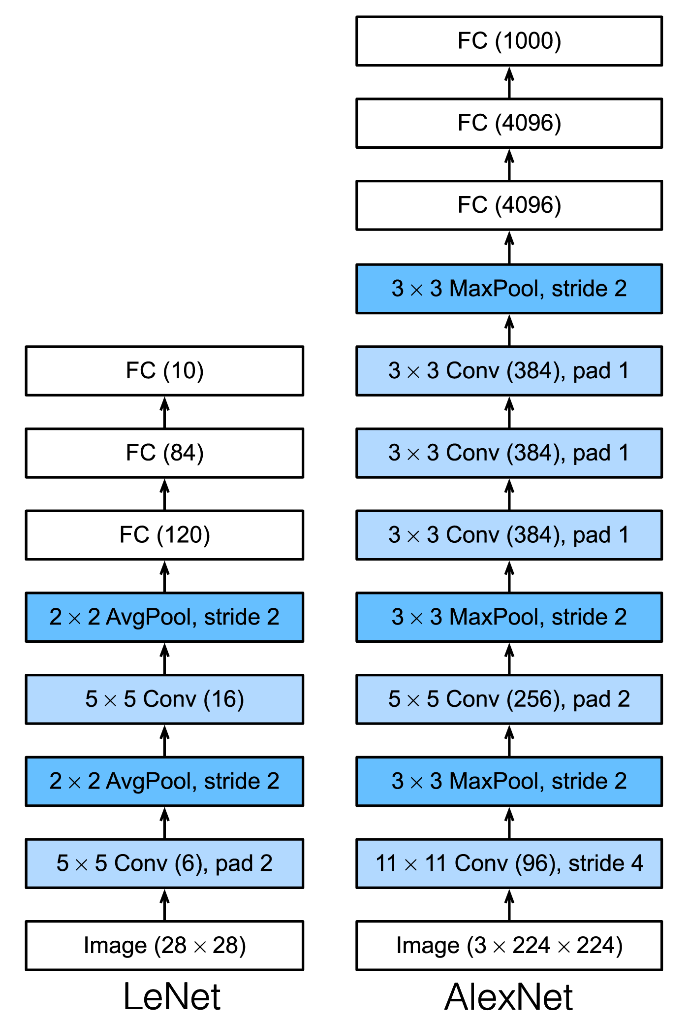
第一,与相对较小的LeNet相比,AlexNet包含8层变换,其中有5层卷积和2层全连接隐藏层,以及1个全连接输出层。下面我们来详细描述这些层的设计。
AlexNet第一层中的卷积窗口形状是11 × 11。因为ImageNet中绝大多数图像的高和宽均比MNIST图像的高和宽大10倍以上,ImageNet图像的物体占用更多的像素,所以需要更大的卷积窗口来捕获物体。第二层中的卷积窗口形状减小到5 × 5,之后全采用3 × 3。此外,第一、第二和第五个卷积层之后都使用了窗口形状为3 × 3、步幅为2的最大池化层。而且,AlexNet使用的卷积通道数也大于LeNet中的卷积通道数数十倍。
紧接着最后一个卷积层的是两个输出个数为4096的全连接层。这两个巨大的全连接层带来将近1 GB的模型参数。由于早期显存的限制,最早的AlexNet使用双数据流的设计使一个GPU只需要处理一半模型。幸运的是,显存在过去几年得到了长足的发展,因此通常我们不再需要这样的特别设计了。
第二,AlexNet将sigmoid激活函数改成了更加简单的ReLU激活函数。一方面,ReLU激活函数的计算更简单,例如它并没有sigmoid激活函数中的求幂运算。另一方面,ReLU激活函数在不同的参数初始化方法下使模型更容易训练。这是由于当sigmoid激活函数输出极接近0或1时,这些区域的梯度几乎为0,从而造成反向传播无法继续更新部分模型参数;而ReLU激活函数在正区间的梯度恒为1。因此,若模型参数初始化不当,sigmoid函数可能在正区间得到几乎为0的梯度,从而令模型无法得到有效训练。
第三,AlexNet通过丢弃法(Dropout)来控制全连接层的模型复杂度,避免过拟合。而LeNet并没有使用丢弃法。
第四,AlexNet引入了大量的图像增广,如翻转、裁剪和颜色变化,从而进一步扩大数据集来缓解过拟合。
下面是一个使用PyTorch实现的稍微简化过的AlexNet。这个网络假设使用1 × 224 × 224的输入,即输入只有一个通道,比如Fashion-MNIST这样的黑白单颜色的数据集。
class AlexNet(nn.Module):
    def __init__(self):
        super(AlexNet, self).__init__()

        # convolution layer will change input shape into: floor((input_shape - kernel_size + padding + stride) / stride)
        # input shape: 1 * 224 * 224
        # convolution part
        self.conv = nn.Sequential(
            # conv layer 1
            # floor((224 - 11 + 2 + 4) / 4) = floor(54.75) = 54
            # conv: 1 * 224 * 224 -> 96 * 54 * 54
            nn.Conv2d(in_channels=1, out_channels=96, kernel_size=11, stride=4, padding=1), nn.ReLU(),
            # floor((54 - 3 + 2) / 2) = floor(26.5) = 26
            # 96 * 54 * 54 -> 96 * 26 * 26
            nn.MaxPool2d(kernel_size=3, stride=2),
            # conv layer 2: decrease kernel size, add padding to keep input and output size same, increase channel number
            # floor((26 - 5 + 4 + 1) / 1) = 26
            # 96 * 26 * 26 -> 256 * 26 * 26
            nn.Conv2d(in_channels=96, out_channels=256, kernel_size=5, stride=1, padding=2), nn.ReLU(),
            # floor((26 - 3 + 2) / 2) = 12
            # 256 * 26 * 26 -> 256 * 12 * 12
            nn.MaxPool2d(kernel_size=3, stride=2),
            # 3 consecutive conv layer, smaller kernel size
            # floor((12 - 3 + 2 + 1) / 1) = 12
            # 256 * 12 * 12 -> 384 * 12 * 12
            nn.Conv2d(in_channels=256, out_channels=384, kernel_size=3, stride=1, padding=1), nn.ReLU(),
            # 384 * 12 * 12 -> 384 * 12 * 12
            nn.Conv2d(in_channels=384, out_channels=384, kernel_size=3, stride=1, padding=1), nn.ReLU(),
            # 384 * 12 * 12 -> 256 * 12 * 12
            nn.Conv2d(in_channels=384, out_channels=256, kernel_size=3, stride=1, padding=1), nn.ReLU(),
            # floor((12 - 3 + 2) / 2) = 5
            # 256 * 5 * 5
            nn.MaxPool2d(kernel_size=3, stride=2)
        )
        # fully connect part
        self.fc = nn.Sequential(
            nn.Linear(256 * 5 * 5, 4096),
            nn.ReLU(),
            # Use the dropout layer to mitigate overfitting
            nn.Dropout(p=0.5),
            nn.Linear(4096, 4096),
            nn.ReLU(),
            nn.Dropout(p=0.5),
            # Output layer.
            # the number of classes in Fashion-MNIST is 10
            nn.Linear(4096, 10),
        )

    def forward(self, img):
        feature = self.conv(img)
        output = self.fc(feature.view(img.shape[0], -1))
        return output
模型训练
虽然论文中AlexNet使用ImageNet数据集,但因为ImageNet数据集训练时间非常长,我们使用Fashion-MNIST数据集来演示AlexNet。读取数据的时候我们额外做了一步将图像高和宽扩大到AlexNet使用的图像高和宽224。这个可以通过torchvision.transforms.Resize实例来实现。也就是说,我们在ToTensor实例前使用Resize实例,然后使用Compose实例来将这两个变换串联以方便调用。
def load_data_fashion_mnist(batch_size, resize=None, root='~/Datasets/FashionMNIST'):
    """Use torchvision.datasets module to download the fashion mnist dataset and then load into memory."""
    trans = []
    if resize:
        trans.append(torchvision.transforms.Resize(size=resize))
    trans.append(torchvision.transforms.ToTensor())

    transform = torchvision.transforms.Compose(trans)
    mnist_train = torchvision.datasets.FashionMNIST(root=root, train=True, download=True, transform=transform)
    mnist_test = torchvision.datasets.FashionMNIST(root=root, train=False, download=True, transform=transform)
    if sys.platform.startswith('win'):
        num_workers = 0
    else:
        num_workers = 4
    train_iter = torch.utils.data.DataLoader(mnist_train, batch_size=batch_size, shuffle=True, num_workers=num_workers)
    test_iter = torch.utils.data.DataLoader(mnist_test, batch_size=batch_size, shuffle=False, num_workers=num_workers)

    return train_iter, test_iter
load_data_fashion_mnist()方法定义了读取数据的方式,Fashion-MNIST原来是1 × 28 × 28的大小。resize在原图的基础上修改了图像的大小,可以将图片调整为我们想要的大小。
def train(net, train_iter, test_iter, batch_size, optimizer, num_epochs, device=mlutils.try_gpu()):
    net = net.to(device)
    print("training on", device)
    loss = torch.nn.CrossEntropyLoss()
    timer = mlutils.Timer()
    # in one epoch, it will iterate all training samples
    for epoch in range(num_epochs):
        # Accumulator has 3 parameters: (loss, train_acc, number_of_images_processed)
        metric = mlutils.Accumulator(3)
        # all training samples will be splited into batch_size
        for X, y in train_iter:
            timer.start()
            # set the network in training mode
            net.train()
            # move data to device (gpu)
            X = X.to(device)
            y = y.to(device)
            y_hat = net(X)
            l = loss(y_hat, y)
            optimizer.zero_grad()
            l.backward()
            optimizer.step()
            with torch.no_grad():
                # all the following metrics will be accumulated into variable `metric`
                metric.add(l * X.shape[0], mlutils.accuracy(y_hat, y), X.shape[0])
            timer.stop()
            # metric[0] = l * X.shape[0], metric[2] = X.shape[0]
            train_l = metric[0]/metric[2]
            # metric[1] = number of correct predictions, metric[2] = X.shape[0]
            train_acc = metric[1]/metric[2]
        test_acc = mlutils.evaluate_accuracy_gpu(net, test_iter)
        if epoch % 1 == 0:
            print(f'epoch {epoch + 1} : loss {train_l:.3f}, train acc {train_acc:.3f}, test acc {test_acc:.3f}')
    # after training, calculate images/sec
    # variable `metric` is defined in for loop, but in Python it can be referenced after for loop
    print(f'total training time {timer.sum():.2f}, {metric[2] * num_epochs / timer.sum():.1f} images/sec ' f'on {str(device)}')
在整个程序的main()方法中,先定义网络,再使用load_data_fashion_mnist()加载训练和测试数据,最后使用train()方法进行模型训练:
def main(args):

    net = AlexNet()
    optimizer = torch.optim.Adam(net.parameters(), lr=args.lr)

    # load data
    train_iter, test_iter = mlutils.load_data_fashion_mnist(batch_size=args.batch_size, resize=224)
    # train
    train(net, train_iter, test_iter, args.batch_size, optimizer, args.num_epochs)

if __name__ == '__main__':
    parser = argparse.ArgumentParser(description='Image classification')
    parser.add_argument('--batch_size', type=int, default=128, help='batch size')
    parser.add_argument('--num_epochs', type=int, default=10, help='number of train epochs')
    parser.add_argument('--lr', type=float, default=0.001, help='learning rate')
    args = parser.parse_args()
    main(args)
其中,args为参数,可以在命令行中传递进来。
我将源代码上传到了GitHub上,并提供了PyTorch和TensorFlow两个版本。
小结
- AlexNet跟LeNet结构类似,但使用了更多的卷积层和更大的参数空间来拟合大规模数据集ImageNet。它是浅层神经网络和深度神经网络的分界线。
- AlexNet现在已经被各种新的模型超越,但仍然是一个里程碑。
- 虽然看上去AlexNet的实现比LeNet的实现也就多了几行代码而已,但这个观念上的转变和真正优秀实验结果的产生令学术界付出了很多年。究其原因,数据、算力曾是深度学习的瓶颈。
- Dropout、ReLU等技术的引入也提升了计算机视觉的性能。
参考资料
- Krizhevsky, A., Sutskever, I., & Hinton, G. E. (2012). Imagenet classification with deep convolutional neural networks. In Advances in neural information processing systems (pp. 1097-1105).
- http://d2l.ai/chapter_convolutional-modern/alexnet.html
- https://tangshusen.me/Dive-into-DL-PyTorch/#/chapter05_CNN/5.6_alexnet